Hamming bird from Ctrl-Space CTF 2025 - Writeup and making of

Last week-end the Ctrl+Space CTF Quals took place. It was a CTF sponsored by the European Space Agency and organized by the mHACKeroni CTF team, and I had the pleasure of developing several challenges for the radio category together with my teammate @marcogpt.

For this CTF we built three different challenges with the following concepts:

• Hamming bird: a common radio reverse-engineering challenge — just an IQ file with a message buried inside and almost no hints on what to do.
• stack-building: the concept was to deploy a virtual satellite and ask users to build a communication pipeline to correctly decode messages from it and encode messages to send to it. The stack was (almost) the same as the one described in the CCSDS Blue Books; various taps were provided to help users debug the different stages of the pipeline
• stack-smashing: using the communication stack developed in the previous challenge, participants were asked to actually pwn the software deployed on the virtual satellite

Writeup

A flying bird is transmitting some telemetry data; check if any important information has been broadcast!

The given attachment was a 133MB raw RF dump, collected somehow, called rf-dump.complex.

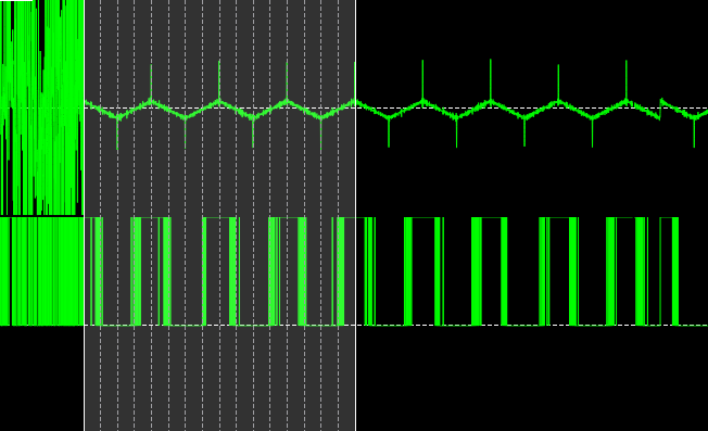
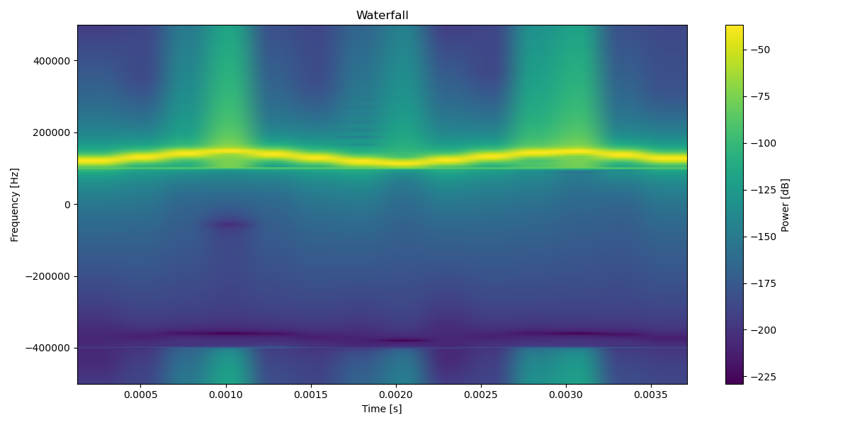
The first thing I like to do when I have an RF dump is open it in inspectrum and try to guess the modulation, symbol period, sample rate, and more — just by looking at its signal spectrum:

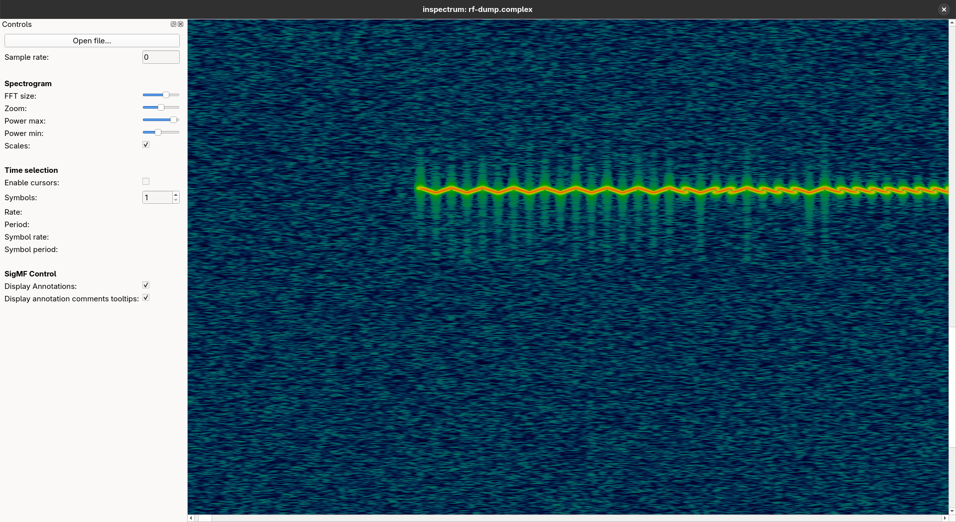
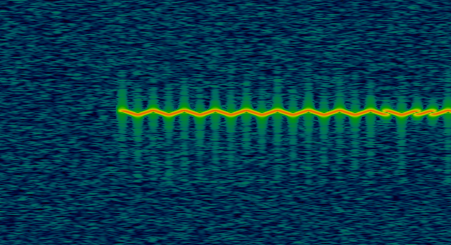
After tweaking Power max and Power min a bit, it is possible to notice a nice signal that doesn’t start right at the beginning of the dump:

The Inspectrum tool shows a spectrogram (waterfall) in which:

• the time domain is on the \(x\) axis,
• the frequency domain is on the \(y\) axis,
• the power of the signal at a specific time and frequency is expressed by the color of the image.

The modulation appears to change the transmission frequency linearly up and down based on the bitstream — i.e., a frequency sweep that encodes data.

To make some measurements we need to enter a sample rate into Inspectrum. Let’s use 100k as an example, then enable the cursor feature. We can drag the selector that appears on the plot and use it to measure how long the sweep lasts:

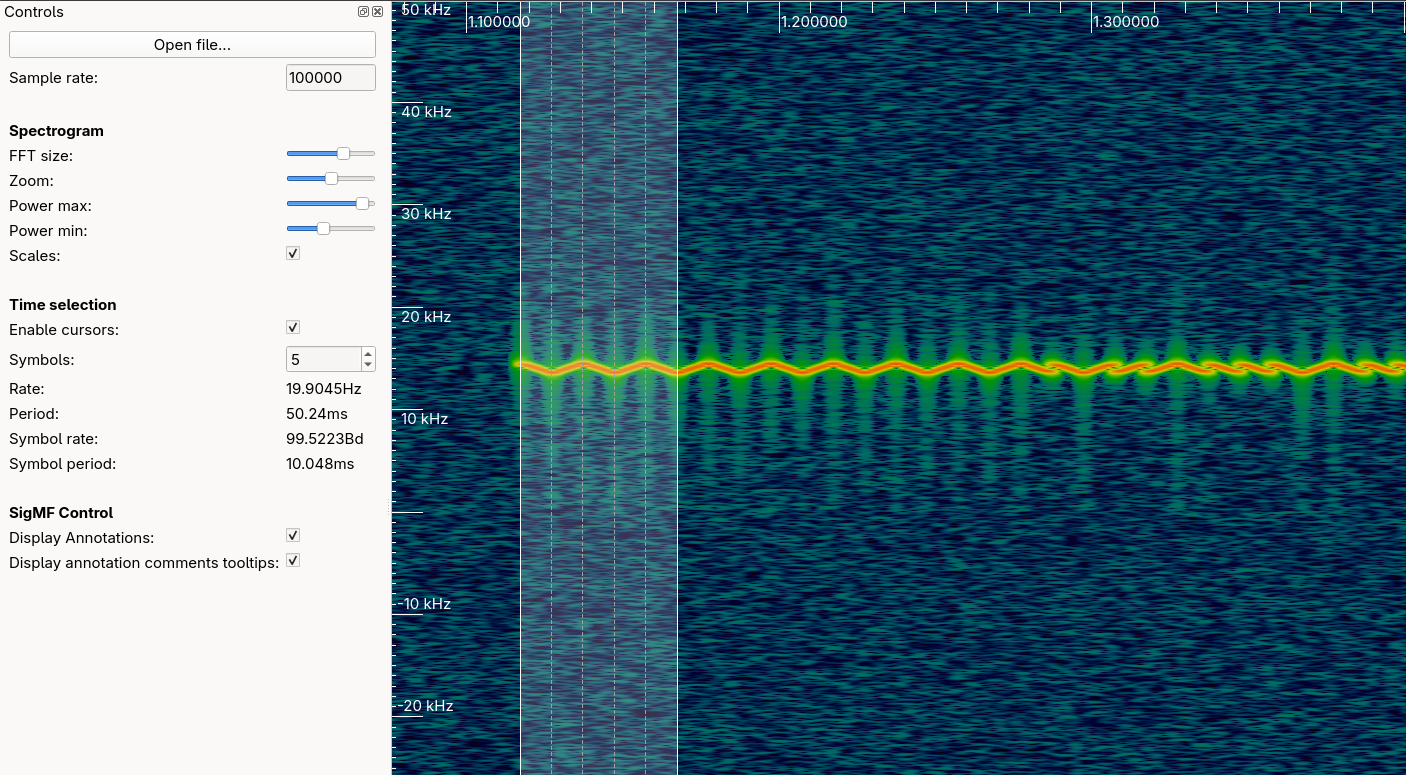
At a sample rate of 100k we can say each symbol lasts 10ms. Of course we can’t be certain the sample rate is correct, but we don’t necessarily need the exact rate to decode the signal, so we’ll proceed with this estimation.

Demodulation (the quick way)

To extract the encoded bits as quickly as possible, we can use Inspectrum directly.
The tool has built-in functionalities to extract amplitude, frequency, and phase components by creating a derived plot.

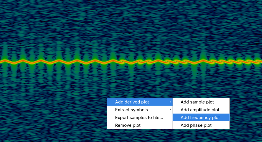
By creating a derived plot from the frequency, it becomes possible to add a threshold plot.
This threshold essentially squares the signal depending on whether the frequency is above or below the chosen value. Then we can use the extract symbols feature.

For coherent symbol recovery, we can set the cursor to a symbol period of 5ms. In this setup:

• an increasing sweep is decoded as 01 (the first half of the symbol is below the threshold, the second half above),
• a decreasing sweep is decoded as 10.

Extracting 16 symbols in this configuration gives the following output:

1, 0, 0, 1, 1, 0, 0, 1, 1, 0, 0, 1, 1, 0, 0, 1

which is coherent with the plot who has alternate decreasing and increasing sweeps.

Looking again at the entire dump, we can see several transmission bursts separated by silence. From this, we can deduce the concept of a frame as a transmission unit. The first frame measures 1824 symbols long, which corresponds to 912 bits, or 114 bytes. The other frame seems to be the same as well.

Demodulation (the nice way)

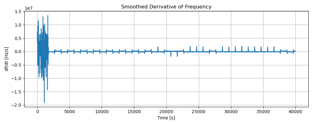
A more formal way to recover the bitstream is to recover the frequency, just like inspectrum does, and then take the derivative of the instantaneous frequency. Given that the frequency is a linear component, the derivative will be a flat line, when the frequency increases the derivative will be positive, instead when the frequency decreases the derivative will be negative.

Having this structure it is possible to just use the sign of the derivative to decide the bit.

The python notebook showing the full process can be seen here, however let’s discuss the main steps without the code.

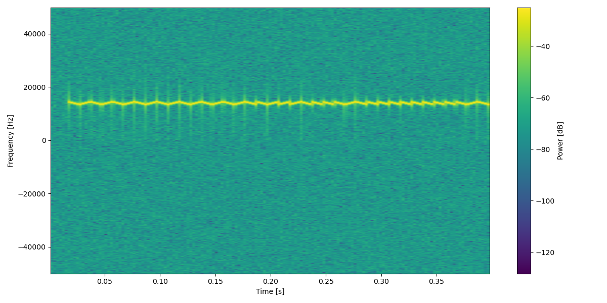
• We’ve already seen the signal structure on inspectrum, but as a reference we can plot it too using matplotlib.pyplot.specgram:
• it can be noticed that the signal is not centered around the \(x=0\) axis, this could make our filtering a bit more tricky, so let’s move it down. This can be done multipying the target signal to a complex exponential of the type:

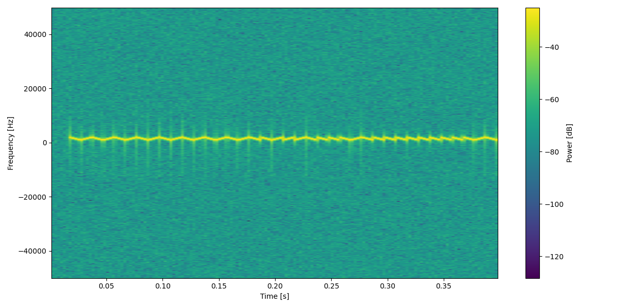
• so far so good, but in order to work with the signal it is useful to filter out unwanted components, since we moved the signal to be around zero we can use a low pass filter with a badwidth of 15kHz:

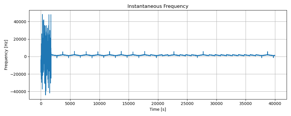
• the main step of the decoding is the extraction of the instantaneous frequency from the signal. This can be achieved using numpy builtins:
  • np.angle to extract the phase of each sample
  • np.unwrap to unwrap the phase from the usual domain \([-\pi, \pi]\)
  • np.diff to compute the derivative of the phase, which is the frequency

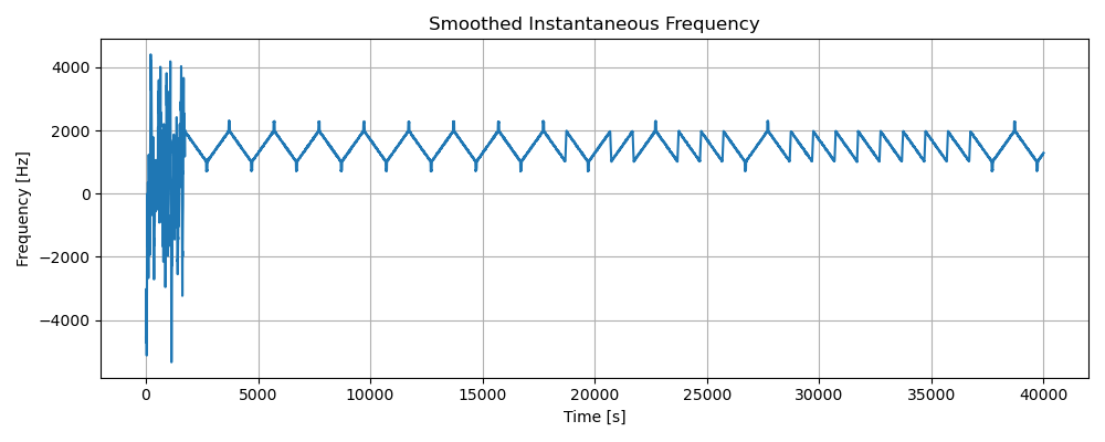
• before taking the derivative of the frequency it is useful to smooth out the signal to remove further noise and act on various outliers, mainly present when the transmission is not active. So after a moving average we get a more ideal signal:

• then we can compute the derivative and gain a square like signal:

• which can in the end under-sampled in order to recover the transmitted bits:

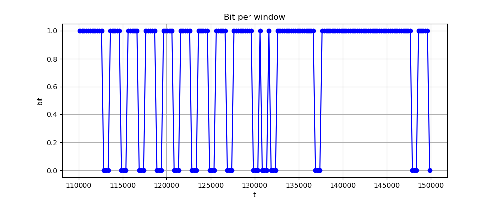
A useful thing to do in those cases is to compute more than 1 symbol for each bit of the transmission, in this case we started with 1000 samples for each transmitted symbol, then undersampled to 4 samples per transmitted symbol, as can be noticed from the plot.

This can be useful during the preamble lookup because we can compare the over-sampled signal to a over-sampled preamble and use a correlation score to decide when a frame could start, instead of looking for an exact match, which could not always be the case.

Note to myself: downsampling

If you want to work with fewer samples (and therefore use less memory), you can use a process called decimation. This is a resampling method that returns the signal as if it had originally been sampled at a lower rate. This process loses information, however for signals with a long symbol period, this is not a major concern.

What you should be careful about, instead, is the decimation factor: choosing a factor that makes the symbol period a fractional number of samples can cause problems when recovering symbols. This is because during recovery we’ve tried to build bits using a fixed number of samples. With a fractional number, however, significant shifts occur, which can desynchronize our windows and mix up bits during the decision process.

Therefore, it is always a good idea to check the symbol period and its relation to the sample rate. Alternatively, you can perform a dynamic decision process that does not rely on a fixed sample window to decide the symbols.

Decoding

Once the bitstream has been recovered, we need to decode the bits and assign them some meaning.

Naively packing the obtained bits gives us useless output, such as:

b'\xaa\xaa\xc7\xbf\xf5\x80$\x08@\x08\x1f\xbd\xf4\xf0\xaek'
b'\x8a\xaa\xa6\xff\xac\x80\x08\x00\x84@;\xf3\xf6\xb2\xf6h'
b'\xaa\xaa\x83\xfb\xdd(\x08\x08\x02\x10:\xfe\xf40bk'
b'\xaa\xaa\x97\xdf\xbd(\x00\xa0\x02\x089\xfb\xf4\xf8\xe7I'
b'\xaa\xaa\x96\xfe\xfd(\x01\x08\x10\x11?\xf3\xf4\x98\xeeI'

Although the data shows some coherence and repeating patterns, it has no clear meaning. However, we can conclude a few things:

• The initial pattern formed by AAAA bytes is likely a sync marker used by hardware to detect the start of a signal.
• The data is most likely not encrypted — otherwise, most of it would change to introduce the diffusion and confusion expected from cryptographic schemes.
• The repeating patterns are sometimes broken by small bit flips, suggesting the presence of errors. These could come either from our demodulation method or from the communication itself.

Recalling the challenge name, Hamming bird, an educated guess would be that it involves some form of error correction based on Hamming code.

Without going into detail on how Hamming codes work, by looking up various implementations (or kindly asking ChatGPT) and performing some trial and error, we can determine that the algorithm used is Hamming (7,4).

Applying this algorithm, we end up with the following output:

b'?\xfa\x00\x00\x07\xffSAT=NIGHTINGALE;TEMP=22.4C;VOLT=3.31V;STATUS=NOMINAL\x00\x00\x00\x00)\xd2'
b'?\xd4\x00\x00\x07\xffSAT=\xceIGHTINGANE;TEMP=22.7C\x0bVOLT=3.29V;STATUS=NOMINAL\x00\x00\x00\x00`\xb6'
b'?\xfa\x00\x00\x07\xffSAT=NIGHTINGALE;T\xd5MP=23.1C;VOLT=3.28V;STATUS=NOMINDL\x00\x00\x00\x00\x0e\xd0'
b'?\xfa\x00\x00\x07\xffSAT=NIGHTINGALE;STATUS=space{1t_w4s_i_4n_h4mming_bird?}\x00\xc4 '
b'?\xfa\x00\x00\x07\xffSAT4NIGHTINGALE;TEMP=23.5C;VOLT=3.30V;STATUS=GOMINAL\x00\x00\x00\x009G'

And in the fourth packet, we find the flag: space{1t_w4s_i_4n_h4mming_bird?}

Making of

The original idea of this challenge was to somehow mimic the LoRa protocol, which uses chirp spread spectrum modulation to achieve low power consumption and robustness against noise.

To add a step after demodulation (and probably introduce some guessing — sorry :)), we decided to include error correction in the communication and chose the Hamming code (7,4).

Generating a chirp

Let’s start by deriving a formula for the chirp. A chirp is a sinusoid whose frequency increases (or decreases) over time. We’ll use a linear increase with respect to time, so a formal definition could be:

where:

• \(f_s\): the starting frequency of the chirp
• \(m\): a coefficient that determines how quickly the frequency increases

To generate our chirp, we used a few shortcuts out of convenience:

• we fixed the sample rate and the symbol time (from this, the baud rate can be calculated as the inverse of the symbol time)

• given the sample rate and symbol time, we can calculate how many samples are needed for each symbol we want to transmit. We’ll refer to this as sps from now on:

• we then created a linear ramp from 0 to 1 whose length is exactly one symbol (the down-chirp is just the reverse of the up-chirp)

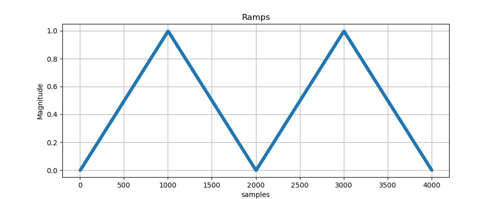
• finally, we used the ramp as the \(mt\) component, scaled by a \(\delta\) that represents the maximum deviation from the initial frequency:

zero = np.arange(0, 1, 1/sps)                   # ramp up
zero_phase = (fs + delta*zero) * symbol_t       # phase of the chirp
modulated = np.cos(2 * np.pi * zero_phase)      # actual chirp

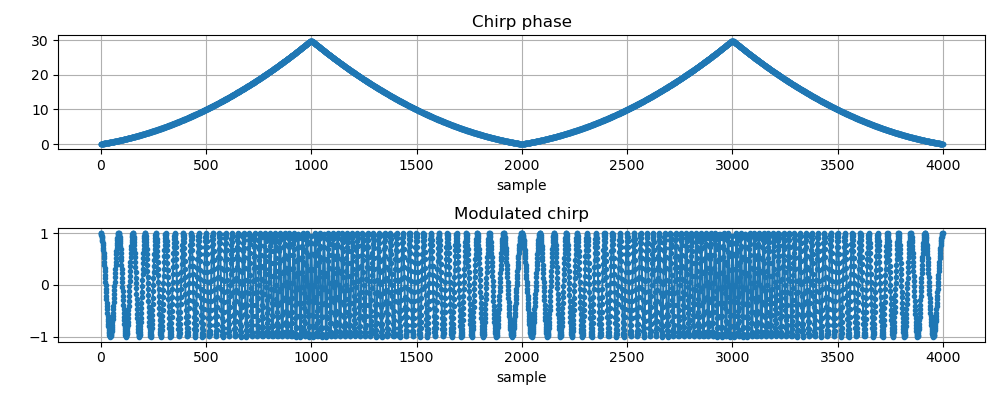
By doing some cut-and-paste, it is possible to encode arbitrary bits using the generated up- and down-chirps.

Make it complex

Looking at the spectrogram of the generated signal, it is possible to notice that it is symmetric around the 0 frequency:

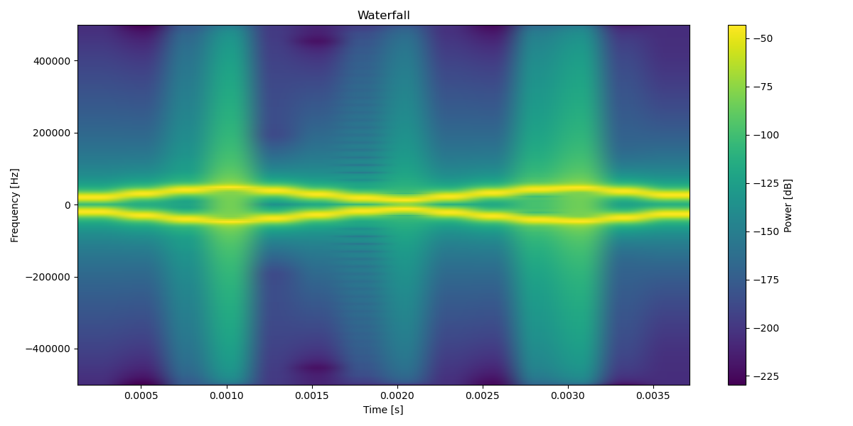
This happens because the signal is real, and due to the Hermitian symmetry of the Fourier Transform:

the Fourier Transform is symmetric.

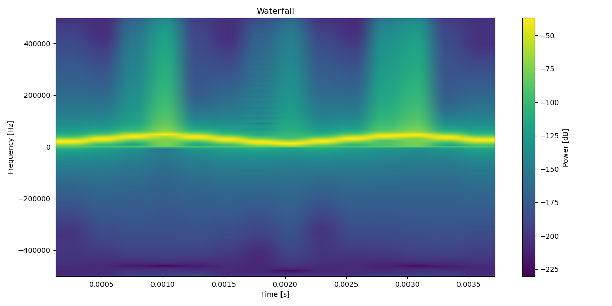
To avoid this symmetry, we need to make the signal complex, but without altering the encoded information too much.
The Hilbert Transform can be used for this purpose.

The Hilbert Transform is an operator that applies a 90° phase rotation to the Fourier Transform of a signal:

Let’s consider the analytic signal:

Then its Fourier Transform is:

In other words, the positive frequencies are doubled, while the negative ones disappear entirely.

Looking at the documentation of scipy.signal.hilbert, that is exactly what happens:

The analytic signal is calculated by filtering out the negative frequencies and doubling the amplitudes of the positive frequencies in the FFT domain. The imaginary part of the result is the hilbert transform of the real-valued input signal.

Shipping the challenge

Last steps before shipping the challenge:

• shift up the signal:

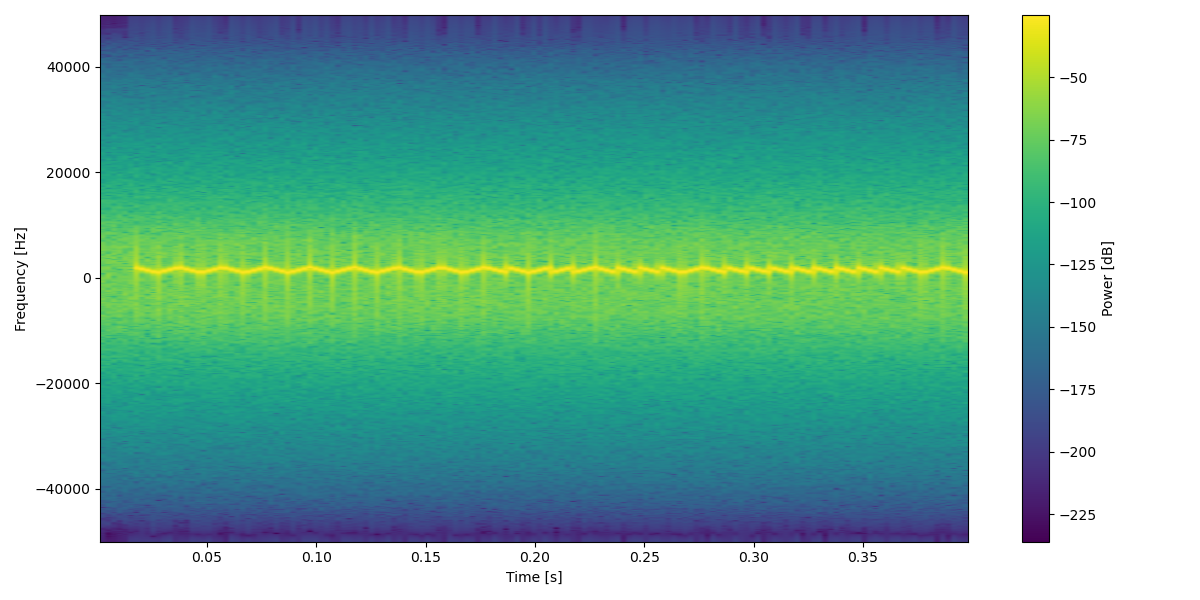
• add noise:

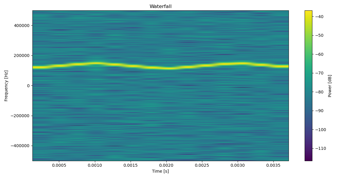
The python notebook detailing all the steps can be found here.

Acknowledgements

I would like to sincerely thank @marcogpt for helping me with some tricky steps, as well as all the participants of the CTF!